Water Hammer in Excel

This Excel spreadsheet will calculate the maximum pressure surge when the valve at the end of a pipeline is closed.

When flow is suddenly stopped, flow inertia causes a pressure surge at the valve, with a shockwave propagating through the pipeline.  This  is also known as Water Hammer and can cause considerable damage.  Engineers need to know the maximum pressure surge to correctly design the pipe, valve andother fittings.

Water hammer is a common phenomenon. For example, the audible creaking when taps are shut off in kitchens or bathrooms results from the Water Hammer effect


These are the equations implemented in the spreadsheet.

where

  • K is the bulk modulus of the liquid (Pa)
  • ρ is the liquid density (kg m -3)
  • D is the pipe diameter (m)
  • t is the pipe wall thickness (m)
  • E is the Young's Modulus of the pipe (Pa)
  • c is the speed of sound in the pipe (m s-1)
  • Δv is the velocity of the liquid before the valve is shut  (m s-1)
  • ΔP is the maximum pressure (at the valve) generated by the valve closure(Pa)

Δv can be easily calculated by the Darcy-Weisbach equation. ΔP is also known as the Joukowsky Pressure.

These equations do not predict the pressure surge arising from column separation (which may be higher than the Joukowsky Pressure). Column separation references the breaking of liquid columns in filled pipes.

Download Excel Spreadsheet for Water Hammer

Dynamic Liquid Flow Between Coupled Tanks

This Excel spreadsheet models the transient flow of liquid between two tanks connected by a pipe.  Because of the momentum of the liquid, the height of liquid in each tank oscillates to an equilibrium.  Flow is opposed by pipe friction, and eventually the liquid level in each tank stabilises.


The dynamics are defined by the following differential equations, which are derived from a mass balance and momentum balance (ref: "Chemical Engineering Dynamics: An Introduction to Modelling and Computer Simulation" by John Ingham et al).


  • H1(t) and H2(t) are the height of liquid in each tank
  • A1 and A2 are the cross-sectional area of each tank
  • Q is the flowrate in the pipe (m3 s-1
  • ρ is the liquid density (kg m-3)
  • μ is the liquid viscosity (Pa s)
  • g is the gravitational constant (9.81 m s-2)
  • L is the length of the pipe (m)
  • D is the pipe diameter (m)
  • e is the pipe roughness (m)
  • Re is the Reynolds number
  • f is the friction factor (for Re < 2000, f is given by 64/Re, while for Re ≥ 2000 f is given by the Haaland equation)
The differential equations are solved in Excel with a simple finite difference Euler scheme, as described by these equations

The spreadsheet is straightforward to use.  Simply enter your parameters.


The spreadsheet will then calculate the flowrate in the pipe, and the change in liquid height in each tank over time. Note that the first row of the results (at t=0) contain the initial conditions.  These can be changed.


The spreadsheet also plots the liquid height in each tank over time.  As you can see, the level of each tank oscillates over time, with the flow being damped by friction.  Eventually,  the height of liquid in each tank reaches an equilibrium level.


Darcy-Weisbach Equation for Liquid Velocity in a Pipe

This Excel spreadsheet uses the Darcy-Weisbach equation to calculate liquid velocity in a pipe.  The Darcy-Weisbach equation describes the relationship between the pressure loss and liquid velocity in a pipe.

This is the equation employed in the spreadsheet.


  • ΔP is the pressure loss in the pipe (Pa)
  • ρ is the liquid density (kg m-3)
  • μ is the liquid viscosity (Pa s)
  • g is the gravitational constant (9.81 m s-2)
  • L is the length of the pipe (m)
  • D is the pipe diameter (m)
  • V is the liquid velocity (m s-1)
  • f is the Darcy Fanning friction factor
For laminar flow (Re<2000), the friction factor f is 64/Re (where Re is the Reynolds Number). Ror turbulent flow the friction factor is given by the Haaland equation (although the Colebrook equation can be used instead).


The calculation is iterative, and requires the use of Excel's Goal Seek. However, this is automated in the spreadsheet so you only have to click a button and some VBA initiates Goal Seek for you.


The Darcy-Weisbach equation should only be used for steady-state incompressible flow. It can also be used for open-channel flows by replacing the diameter with the 4 R, where R is the hydraulic diameter.  The hydraulic diameter is simply the cross-sectional area divided by the wetted perimeter.


TEMA Type E Heat Exchanger Design

This Excel spreadsheet helps you design a TEMA Type E heat exchanger. The spreadsheet uses the Bell-Delaware method to calculate the overall heat transfer coefficient and the shell-side pressure drop.

TEMA Type E heat exchangers are the basis of many other designs. They offer a single pass, with liquid entry and exist on opposing sides of the shell

The spreadsheet allows you to pick from a triangle, square or rotated square tube placement, and specify the precise geometry of the shell, and then calculates the shell-side pressure drop and heat transfer coefficient accordingly.

The spreadsheet contains several empirical correlations, including those to calculate the Colburn J factor (used in determining the shell-side friction factor) and the pressure drop.


In the Bell-Delaware method, the shell-side heat transfer coefficient is the ideal heat transfer coefficient for cross-flow across a tube bank, multiplied by several correction factors as follows


The correction factors adjust the ideal heat transfer coefficient for leakage effects, bundle bypass, baffle spacing, and baffle cut. The correction factors are all calculated inside the spreadsheet for your convenience. The product of all the correction factors are equal to about 0.6 for an efficiently designed heat exchanger.

The spreadsheet is easy to use. Simply enter the process parameters (i.e. flowrates, temperatures, etc) and the geometrical parameters (number of tube passes, shell dimensions etc) in the pink cells.  You will need to equalize heat transfer across the shell-side and tube-side streams by varying a process parameter (this is indicated inside the spreadsheet).

Download Excel Spreadsheet for TEMA Type E Heat Exchanger Design using Bell-Delaware


Temperature Dynamics of Heated Tanks Connected in Series

This Excel spreadsheet models the temperature dynamics of a feed stream heated in three tanks connected in series. Each tank has a heating coil at a fixed temperature, and it is assumed that each tank is perfectly mixed


The temperature dynamics are modeled by these three differential equations.


  • M is the mass of liquid in each tank (kg)
  • T0 is the temperature of the feed stream (K)
  • T1(t), T2(t) and T3(t) are the temperatures in each tank
  • Ts is the temperature of the heating coil
  • W is the flowrate of the feed stream (kg s-1)
  • Cp is the specific heat capacity of the feed stream (J kg-1 K-1)
  • U is the overall heat transfer coefficient (W m-2 K-1)
  • A is the heat transfer area (m2)
The three differential equations were solved analytically to give symbolic equations for the three temperatures T1(t), T2(t) and T3(t) . These  equations were then translated into Visual Basic and implemented in Excel.


The spreadsheet also gives the steady-state temperature Tn of the nth tank connected in series, as predicted by this equation.


Double Pipe Heat Exchanger

This Excel spreadsheet helps you design a double pipe heat exchanger (also known as a concentric tube heat exchanger). Double pipe heat exchangers are often used in the chemical, food processing and oil & gas industries. They have a particular advantage when close temperature approaches are needed or in high pressure applications.

The spreadsheet will give you important design parameters, such as the overall heat transfer area, the length required, pressure drops, fluid velocities and much more.  The spreadsheet uses the
  • Gnielinski correlation for the heat transfer coefficient of the shell side and tube side fluids (hh and hc). The Gnielinski correlation is valid for 0.5 ≤ Pr ≤ 2000 and 2300 ≤ Re ≤ 56.It gives the heat transfer coefficient in terms of the friction factor, the Reynolds number and the Prandtl number.
  • Filonenko correlation for the friction factor (valid for smooth pipes in turbulent flow with 104 ≤ Re ≤ 107).
The equations for the heat transfer coefficients, the friction factor, the length of the heat exchanger and the overall heat transfer coefficient are given below

Double Pipe Heat Exchanger Equations

  • Nu is the Nusselt Number
  • Re is the Reynolds Number
  • f is the friction factor
  • Q is the rate of heat transfer (determined from a heat balance)
  • dic is the internal diameter of the inner pipe
  • doc is the external diameter of the inner pipe
  • kp is the thermal conductivity of the pipe material
  • hc is the heat transfer coefficient of the cold fluid (in the inner pipe)
  • hh is the heat transfer coefficient of the hot fluid (in the outer pipe)
  • ΔTLMTD is the log mean temperature difference
The Excel spreadsheet uses variable names in the formulas to help you better understand the equations. Generally, the suffixes h and c represents quantities defined for the hot and cold streams respectively (e.g. hh is the heat transfer coefficient for the hot stream, hc is the heat transfer coefficient for the cold stream)

Named variables

INSTRUCTIONS

Step 1. Enter your parameters. The spreadsheet will calculate initial values of the heat transfer coefficients, the rate of heat transfer across both fluids, and the length of the heat exchanger. Provide an initial guess for the parameter (i.e. mass flowrate) you will change in Step 2.

Specify your parameters

Step 2. Equalize heat transfer across both streams. The rate of heat transfer across the shell side and tube side fluids must be the same. You must use Goal Seek to make the difference between the two rates of heat transfer equal to zero by changing a design parameter (e.g. mass flowrates)

Goal Seek

You have now established important design parameters, such as the fluid velocities, the tube-side and shell-side pressure drops, Prandtl numbers, the length of the heat exchanger and so on. 

Intermediate Calculations and Results

This spreadsheet is completely free. If you have any comments, then please let me know. Download it from the link below, and please bookmark or share this website wherever you feel it appropriate.


Find Orifice Diameter for Specific Operating Parameters

These Excel spreadsheets will help you find the orifice size for an orifice flow meter, given various design parameters like the desired pressure drop, fluid properties etc. All the spreadsheets use industry-standard designs, such as ISO 5167 and ASME MFC-14M-2001

First, decide what type of orifice you're designing and download the appropriate Excel Spreadsheet (read the articles for the equations and valid operating conditions)

I'll illustrate the calculation process with an example problem (but the principles are the same for the other spreadsheets). All the spreadsheets require Excel's Goal Seek functionality because the calculations are iterative.

We will now find the orifice diameter for a small-bore liquid flow meter under the following conditions
  • Pipe diameter: 0.042m
  • Density: 1000 kg m -3
  • Viscosity: 0.001 Pa s
  • Desired pressure drop: 30 Pa
  • Flange taps
Step 1: Define the parameters as specified above, and also include an initial guess value for the orifice diameter.

Step 2: Go to Data > What If Analysis > Goal Seek. Set the difference in the guess and calculated values of the Reynolds number to zero by varying the orifice diameter.


As soon as you click OK, Excel will give the correct orifice size, as well as other parameters, like the flowrate, orifice coefficients, Reynolds Numbers etc.


Small-Bore Gas Orifice Meter Flow Calculator

This Excel spreadsheet calculates the flowrate from a small-bore gas orifice meter using the ASME MFC-14M-2001 standard. This calculator is valid for pipe diameters of less than 40 mm (other restrictions are given below).


The equations are as follows


  • C is the discharge coefficient. D1 has to be supplied in m
  • D1 and D2 are the diameter of the pipe and orifice respectively (m)
  • A1 and A2 are the cross sectional areas of the pipe and orifice (m2)
  • ΔP is the pressure drop across the orifice (Pa)
  • P1 and Pstd are the upstream pressure and standard pressure
  • T and Tstd are the gas temperature and standard temperature is the 
  • ρ is the gas (kg m-3)
  • μ is the gas viscosity (Pa s)
  • V1 is the liquid velocity in the pipe (m s-1)
  • Re1 is the Reynolds Number in the pipe
  • β is the diameter ratio
  • MW is the molecular weight of the gas (kg mol-1)
  • R is the universal gas constant (8314 J kmol-1 K-1)
  • γ is the specific heat ratio
  • e is the gas expansivity
  • Q is the volumetric flowrate (m3s-1)
  • Qstd is the volumetric flowrate at standard conditions (m3s-1)
The spreadsheet uses the ideal gas law to calculate the gas density (you just have to supply the molecular weight, pressure and temperature of the gas).

Note these restrictions to the validity of the equations
  • Corner Taps: 0.1 < β < 0.8 and 12 mm < D< 40 mm
  • Flange Taps: 0.15 < β < 0.7 and 25 mm < D< 40 mm
  • D2 > 6 mm
  • Re >1000
Additionally, the discharge coefficients are only valid for the tap configurations illustrated below (as specified by the ASME MFC-14M-2001 standard).


You can choose either Corner or Flange taps with a drop-down menu in the spreadsheet, and Excel automatically uses the correct correlation for the discharge coefficient.

These equations (like nearly all orifice flow meter calculations) require an iterative solution. This is easily done with Excel's Goal Seek.  All you have to do is click a button.

Goal Seek uses an initial guess value for the Reynolds Number to calculate the discharge coefficients, and uses this to calculate the flowrate. The calculated flowrate is then used to calculate the Reynolds Number.  Goal Seek then automatically adjusts the guess and calculated values of the Reynolds number until they are the same.


Small-Bore Liquid Orifice Flow Meter Calculator for Excel

This Excel spreadsheet calculates the liquid flowrate from a small-bore orifice meter using the equations defined in ASME MFC-14M-2001. The calculation is iterative, but the spreadsheet is conveniently set up to use Excel's Goal Seek functionality by simply clicking a button.


The equations implemented in the spreadsheet are sourced from ASME MFC-14M-2001 and are given below.


The notation is given below.
  • C is the discharge coefficient. D1 must be supplied in m.  The equation differs for flange taps and corner taps, but a menu in the spreadsheet allows you to pick between the two.
  • D1 and D2 are the diameter of the pipe and orifice respectively (m)
  • A1 and A2 are the cross sectional areas of the pipe and orifice (m2)
  • ΔP is the pressure drop across the orifice (Pa)
  • ρ is the density of the liquid (kg m-3)
  • V1 is the liquid velocity in the pipe(m s-1)
  • Re1 is the Reynolds Number in the pipe
  • β is the diameter ratio
  • μ is the liquid viscosity (Pa s)
  • Q is the volumetric flowrate (m3s-1)
The correlations for the Flange Taps and Corner Taps discharge coefficient are only valid for the following configurations.


The equations are only valid under the following conditions
  • Corner Taps: 0.1 < β < 0.8
  • Flange Taps: 0.15 < β < 0.7
  • 25 mm < D1 < 50 mm
  • 6 mm < D2 
  • Re > 1000
A β of between 0.3 and 0.7 is practical; below this, the pressure drop is too large for economical operation, and above this, the pressure drop is not large enough for an accurate reading.

The Excel spreadsheet will also calculate the static pressure loss and the head loss from a distance D1 upstream and 6 D1 downstream of the orifice.

The spreadsheet is free, and none of the cells are hidden, locked or password protected. Please visit this website regularly for more exclusive, professionally prepared Excel spreadsheets for engineering.

Download Excel Spreadsheet to Calculate Liquid Flow from a Small Bore Orifice Meter


Critical Oil Flowrate for Gas Coning


This Excel spreadsheet uses the Mayer and Garder correlation to calculate the oil flowrate necessary to form a stable gas cone in an oil and gas reservoir.

Gas coning references the tendency of gas to flow in the direction in which its face the least resistance, against the flow of gravity.  Above the critical oil flowrate, the cone will breakthrough and gas will force the oil flow downwards towards the well perforation.  At this point, gas will tend to dominate crude oil production (often to the point where the well is not economically feasibile).

Gas coning is often significant if an oil reservoir is in contact with an aquifer or gas cap.

The critical oil flowrate is sometimes lower than the economical production rate, but techniques have been developed to combat gas coning (including using horizontal wells instead of vertical wells, and infill drilling)

The Mayer and Garder equation and a screengrab of the spreadsheet are given below.


  • ρo and ρg are the densities of the oil and gas in lb ft-3
  • re and rw are the drainage radius and welbore radius in ft
  • Bo is the oil formation volume factor (this is almost always above 1)
  • μo is the viscosity of the oil in centipoise
  • ko is the effective oil permeability
  • Q is the oil flowrate in stb day-1


  • Calculate Original Gas in Place with Excel

    This Excel spreadsheet calculates the Original Gas in Place with a p/z plot.  Specifically, this spreadsheet fits the observed p/z data and cumulative gas product to the following curve

    where
    • (p/z) is the observed values of pressure over compressibility (collected during the life of a reservoir)
    • Gp is corresponding cumulative gas production (again collected during the life of a reservoir)
    • (p/z)i is the initial value of pressure over compressibility of the system
    • G is the original gas in place
    This equation is simply a material balance, which many engineers use to determine the Original Gas in Place in volumetric natural gas reservoirs. It assumes a constant pore volume and includes the effect of gas expansion.  Note that the equation predicts a linear relationship between p/z and G

    This screen grab illustrates the contents of the spreadsheet.


    The spreadsheet is easy to follow.  It simply minimizes the sum-square residuals (difference between predicted and actual values of p/z) by varying G.  You can also choose to vary (p/z)i in addition to G to minimize the sum-square residuals, but since this value is usually accurately measured, this is not recommended.

    Fundamentally, this method is pretty simple to understand - we're simply locating the intercept on the x-axis (where p/z = 0) of a straight line fit of G against p/z, as illustrated by this picture.


    This method of determining the Original Gas in Place is only suitable for normally pressurized gas reservoirs, where the gas expansion is the only significant factor contributing to gas production. This method, however, is not suitable for abnormally-pressurized reservoirs, where gas production is affected by formation compressibility (i.e.the expansion of sand, rock and water). Gas reservoirs are often abnormally-pressurized if they are in contact with aquifers


    Model a Gas Orifice Meter with Excel

    This Excel spreadsheet calculates the flowrate from the pressure drop across a gas orifice meter with the equations defined in ISO 5167.

    Orifice meters use the pressure loss across a constriction (that is, the orifice plate) in a pipe to determine the flowrate.  While orifice meters are cost effective, they have several disadvantages. 
    • The relationship between flowrate and pressure is non-linear,
    • accurate values of the physical parameters are required,
    • and high Reynolds numbers (>104) are required for the greatest confidence in their accuracy, and the resulting pressure drop can be significant.
    Accordingly, orifice meters are only used with the pressure drop is not critical, and accuracy is around 2% at best.

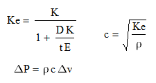
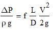
    These are the equations implemented in the spreadsheet (as specified in ISO 5167)

    Gas Orifice Meter Equations in ISO 5167

    The notation is given below
    • C is the discharge coefficient (only valid for the three standard tap positions given below)
    • Re is the Reynolds number
    • L1 and L2 are the upstream and downstream tap positions (m)
    • P1 and P2 are the upstream and downstream pressures (Pa)
    • D1 and D2 are the pipe and orifice diameters (m)
    • V is the gas velocity in the pipe (m s-1)
    • ρ is the gas density (kg m-3)
    • μ is the gas viscosity (Pa s) 
    • M is the molecular weight
    • Y is the expansion coefficient
    • Z is the gas compressibility factor
    • K is the specific heat ratio
    • R is the gas constant (8314 J kg-1 k-1)
    • Ao is the cross-sectional area of the orifice (m2
    There are three standard tap positions that determine the values of L1 and L2, as illustrated below. For corner taps, L1 = L2= 0, for D-D/2 taps L1 = D1 and L2= D1/2, and for flange taps L1 = L2= 1 inch. 
    Tap positions in ISO 5167

    The equations use the ideal gas law to calculate the gas density (you could override this with your own value), and are only valid for pipes with internal diameters from 50 mm to 1000 mm, and for pressure ratios greater than 0.75.

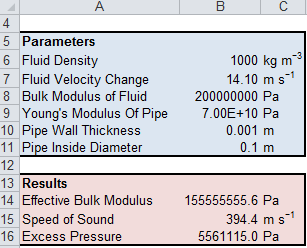
    This is a screen grab of part of the spreadsheet.


    The calculation is iterative: you need Re to calculate C, you need V to calculate Re, but you need C to calculate V.  Excel's Goal Seek functionality is used to iteratively solve the equations for the flowrate. This process is automated with a button - just fill in the parameters, click a button, and some VBA initiates Goal Seek with the correct settings

    The spreadsheet provides an initial guess value for Re. This is used to calculate C and V. V is then used to calculate Re.  Excel's Goal Seek varies the guess value of Re until it matches the calculated value of Re.

    By carefuly altering the equations (and the parameters used by Goal Seek), you could also solve for any other variable - for example, you could find the pressure drop for a specific flowrate (let me know if you need help in implementing this).

    You'll find a spreadsheet  that models a liquid orifice meter here.

    Visit http://excelcalculations.blogspot.com regularly for more free engineering spreadsheets.

    Download Excel Spreadsheet to Calculate Flowrate in a Gas Orifice Meter (ISO 5167)

    Size a Liquid Orifice Meter with ISO 5167 and Excel

    This Excel spreadsheet sizes a liquid orifice meter using the equations in ISO 5167.  Orifice meters determine liquid flowrate by measuring the pressure difference across a constriction in a pipe. 

    The spreadsheet is free - all I ask is that you credit this website with its authorship (and perhaps provide a link!)


    The equations given in ISO 5167 are given below.
    • C is the discharge coefficient (the equation is only valid for the three standard tap positions defined below)
    • Re is the Reynolds number
    • L1 and L2 are the upstream and downstream tap positions (ft)
    • P1 and P2 are the upstream and downstream pressures (psig)
    • D1 and D2 are the pipe and orifice diameters (inches)
    • V is the liquid velocity in the pipe (ft s-1)
    • ρ is the liquid density slugs ft-3
    • μ is the liquid viscosity lb-sec ft-2

    ISO 5167 defines three different tap positions for the pressure probes (Corner, D-D/2 and Flange taps). These positions the values of L1 and L2, and are given below

      • Corner Taps: L1 = L2 = 0
      • Flange Taps: L1 = L2 = 1 inch
      • D-D/2 Taps: L1 = D1, L2 = D1/2
      The solution to the equations is iterative; you need Re to calculate C, but you need Q to calculate Re, but you need C to calculate Q.  This requires the use of Excel's Goal Seek.  We simply find the
      1. Guess a value of Re,
      2. Calculate C and Q
      3. Use C and Q to calculate Re
      4. Use Goal Seek to change the value of Re we guessed in Step 1 until it's equal to the value calculated in Step 3
      This process is automated in the Excel spreadsheet with a button linked to a VBA macro. The VBA macro simply initiates Goal Seek with the requireed settings.

      Download Excel spreadsheet to size an orifice meter with ISO 5167

      Compressibility Factor Calculator for Excel

      This Excel spreadsheet calculates the compressibility factor for natural gas using the Dranchuk-Abou-Kassem correlation.  Engineers need the compressibility factor to calculate natural gas flowrates (e.g., using the Weymouth Equation), viscosities (e.g. using the Lee, Gonzalez and Eakin correlation) or other properties


      Tr is the reduced temperature, Pr is the reduced pressure, and ρr is the reduced density. The correlation is only valid for 0.20 ≤ Pr < 30, and 1.0 < Tr ≤ 30. The constants A1 to A11 were found by a best−fit to the Standing and Katz chart with an average absolute error of 0.585%.


      The Dranchuk-Abou-Kassem equation is implicit; solving for Z requires an iterative solution method.  Several several methods exist in Excel, and the spreadsheet demonstrates two of these methods.
      • A circular reference.  Make sure File>Options>Formulas>Enable iterative calculation is checked)
      • Goal Seek.  Here we 
        • guess a value for Z 
        • use this to calculate ρr
        • use ρr calculate Z
        • use Goal Seek to minimize the difference between the guess and calculated values of Z by varying the guess value of Z
      I've found that the result given via Goal Seek is more numerically stable (the circular reference often gives unrealistic results).  There's a button in the spreadsheet to initiate Goal Seek.

      If you want Goal Seek to automatically recalculate the compressibility factor whenever the reduced temperature or pressure are changed, add this VBA to Sheet1 in the spreadsheet.

      Private Sub Worksheet_Change(ByVal Target As Range)
      Dim bSuccess As Boolean
          On Error Resume Next
          bSuccess = Range("diff").GoalSeek(0, Range("guessz"))
          On Error GoTo 0
          If Not bSuccess Then
              MsgBox "Goal Seek Failed for Compressibility Factor"
          End If
      End Sub

      You may also want to check out this Excel spreadsheet which uses the Beggs and Brill correlation to calculate the compressibility factor of natural gas.

      Download Excel spreadsheet to calculate the compressibility factor with the Dranchuk-Abou-Kassem correlation

      Calculate Erosional Velocity with Excel

      This Excel spreadsheet helps you calculate erosional velocity in Excel.  The offshore oil industry often requires the transport of liquid, gas and solids in long distance pipelines.  This causes the pipe surface to erode, with the rate of erosion increasing with the flow velocity.

      The American Petroleum Institute have guidelines (see API RP14E) for the flow velocity below which erosion damage is minimized.  This maximum flow velocity is a function of velocity and density, and given by this equation.
      where ρ is the gas/liquid density at the flow temperature and pressure, C is an empirical constant, and V is the maximum recommended velocity. This equation is only valid for horizontal flow with shear stress as the limiting factor

      If ρ is in lb ft−3 and V is in ft s−1, then C has units of lb0.5 ft−0.5 s−1. API RP14E recommends that C=100 lb0.5 ft−0.5 s−1 for continuous service of liquid with solids, or C=125 lb0.5 ft−0.5 s−1 for intermittent service (or values of up to 200 lb0.5 ft−0.5 s−1 if the pipelines are corrosion resistant).

      However, recent studies have recommended that higher C values are used, with values of 887 for 13Cr piping for "clean gas service" (see the paper "Improved Procedures for Estimating the Erosional Rates in High Offtake Gas Wells: Applications of University of Tulsa Flow Loop Derived Correlation" for more detail).


      This Excel spreadsheet implements the API RP14E equation to calculate erosional velocity.  If you enter the specific gravity of the liquid and gas components, the gas/liquid volume ratio, the the absolute temperates and pressures, and the compressibility factor, the Excel spreadsheet will calculate the mixture density for you.  Note that the spreadsheet expects all values to be in SI units, including the erosional velocity coefficient C (a conversion factor is supplied in the spreadsheet).


      Calculate Viscosity of Natural Gas with Excel

      This Excel spreadsheet will calculate the viscosity of natural gas. The spreadsheet uses the Lee, Gonzalez and Eakin correlation for the viscosity, and the CNGA (California Natural Gas Association) correlation for the compressibility factor.

      The Lee, Gonzalez and Eakin correlation, only requires the pressure, temperature and molecular weight of the natural gas, and is relatively accurate compared to more complex methods of predicting viscosity.  It still widely used and accepted.

      The CNGA compressibility factor correlation is suitable for pressures above 100 psig (below 100 psig, the compressibility factor is 1)
      The Lee, Gonzalez and Eakin correlation was published in 1964 and accurately predicts the viscosity of natural gases with low non-hydrocarbon content, and for temperature between 100 F - 340 F, and pressures between 14.7-8000 psia. Additionally, the correlation is only suitable for sweet gases, and does not accurately describe sour gases (as described in this paper). The correlation has standard deviation of 2.7%, with a maximum deviation of 8.99%. The correlation is


      Gas density is predicted by this correlation.

      where ρ is the density in g/cm3, P is the pressure in psig, MW is the molecular weight (lb/lbmol), R is the gas constant (10.731 ft3 psi °R−1 lb-mol−1), T is the absolute temperature (°R) and Z is the compressibility factor.


      Calculate Bottom Hole Pressure with the Cullender and Smith Method

      This Excel spreadsheet employs the Cullender and Smith method to calculate Bottom Hole Pressure on a shallow, dry gas well. The bottom hole pressure is simply the pressure at the bottom of an oil-well shaft

      Many reservoir engineering calculations require the static bottom hole pressure.  However, this can be difficult to measure experimentally. A number of researchers have developed other techniques to calculate bottom hole pressure from measurements at the wellhead.

      The Cullender and Smith (1956) method is generally considered accurate and models the variation of compressibility Z with temperature T and pressure P

      This is the Cullender and Smith equation

      It needs to be numerically integrated. In the attached spreadsheet, we have simply divided the entire length into four sections and integrated via a simple trapezoidal method.