This article will develop a dynamic model of a cross-flow heat exchanger from first principles, and then discretize the governing partial differential equation with finite difference approximations. It will then demonstrate how this equation can be implemented in Excel (or indeed any other math tool)

If you just want the Excel implementation, then click here, but I encourage you to read the rest of the article so you understand how the spreadsheet is implemented.
First Principles Modeling
Consider liquid flowing (at mass flowrate F) through a length Δx of pipe (diameter D), subject to cooling by cross-flow air (at temperature Ta and heat transfer coefficient U)

A heat balance over time Δt gives the following.


As Δx and Δt tend to zero, we get the following parabolic partial differential equation
 |
| Equation 1 |
Finite Difference Approximation
A forward difference approximation for the first of temperature with respect to time is
 |
| Equation 2 |
 |
| Equation 4 |
Substituting Equation 2 and 3 into Equation 1, and rearranging gives
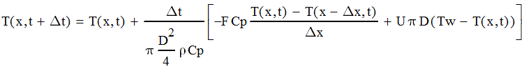 |
| Equation 4 |
We only need to know the temperature of the bar at time t (on the RHS of Equation 4) to calculate the temperature at time t + Δt (on the LHS of Equation 4).
Implementating in Excel
This is how Equation 4 will be implemented in Excel

Step 1 - Specify your parameters, including your chosen time and space step. I've named the cells in Column C with the names in Column E. I'll use named values when entering Equation 4.

Step 2 - Create a column and row containing your space and time steps

Step 3 - Fill in your initial conditions at time t = 0 (this will be the inlet liquid temperature as specified in the parameters).

Step 4 - Insert your boundary conditions at distance x = 0 (this will be the inlet liquid temperature - the same as the initial condition).

Step 5 - Implement Equation 4 into the first empty cell (at t = Δt and x = Δx)

Step 5 - Copy this formula to all other times and positions. For my implementation, I go up to t = 1 and x = 0.4.

The techniques I've demonstrated above can be applied to many other challenges in science, engineering and math. If you have any requests, then let me know.
1 comments:
great work dude......
Post a Comment